
Installation
The latest version can be installed from GitHub with:
devtools::install_github("YsoSirius/windfarmGA")
install.packages("windfarmGA")
Description
The genetic algorithm is designed to optimize wind farms of any shape. It requires a predefined number of turbines, a uniform rotor radius and an average wind speed per wind direction. It can include a terrain effect model, which requires an elevation raster and a surface roughness raster. The elevation data is used to find mountains and valleys and to adjust the wind speeds accordingly by ‘wind multipliers’ and to determine the air densities at rotor heights. The surface roughness raster with an additional elevation roughness value is used to re-evaluate the surface roughness and to individually determine the wake-decay constant for each turbine.
To start an optimization use the function genetic_algorithm.
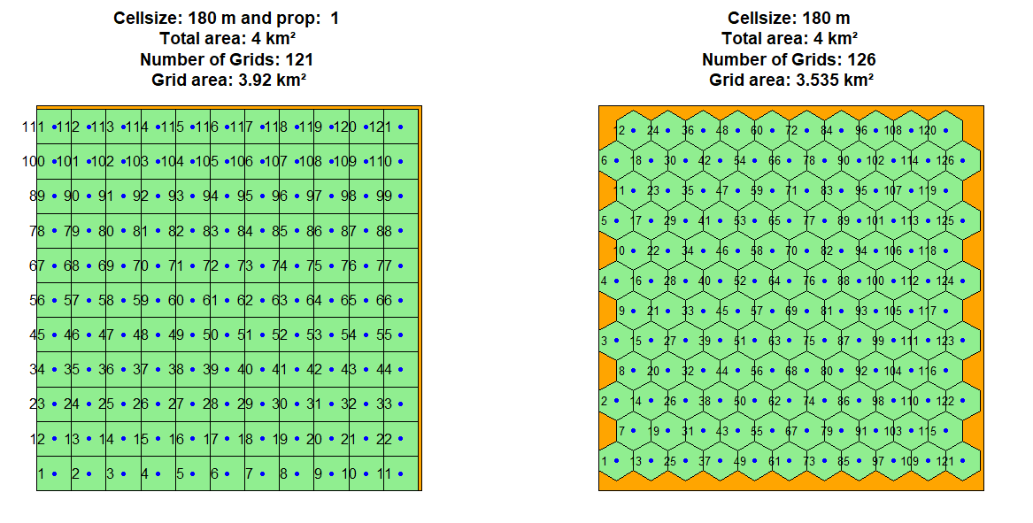
Since version 1.1, hexagonal grid cells are possible, with their center points being possible locations for wind turbines. Furthermore, rasters can be included, which contain information on the Weibull parameters. For Austria this data is already included in the package.
Create an input Polygon
- Input Polygon by source
library(sf)
dsn <- "Path to the Shapefile"
layer <- "Name of the Shapefile"
Polygon1 <- sf::st_read(dsn = dsn, layer = layer)
plot(Polygon1, col = "blue")- Or create a random Polygon
Create random Wind data
- Exemplary input Wind data with uniform wind speed and single wind direction
wind_df <- data.frame(ws = c(12, 12), wd = c(0, 0), probab = c(25, 25))
windrosePlot <- plot_windrose(data = wind_df, spd = wind_df$ws,
dir = wind_df$wd, dirres=10, spdmax = 20)- Exemplary input Wind data with random wind speeds and random wind directions
Grid Spacing
Rectangular Grid Cells
Verify that the grid spacing is appropriate. Adapt the following input variables if necessary: - Rotor: The rotor radius in meters. - fcrR: The grid spacing factor, which should at least be 2, so that a single grid covers at least the whole rotor diameter. - prop: The proportionality factor used for grid calculation. It determines the minimum percentage that a grid cell must cover of the area.
Make sure that the Polygon is projected in meters.
Terrain Effect Model
If the input variable topograp for the functions windfarmGA or genetic_algorithm is TRUE, the genetic algorithm will take terrain effects into account. For this purpose an elevation model and a Corine Land Cover raster are downloaded automatically, but can also be given manually. ( Download a CLC raster ).
If you want to include your own Land Cover Raster, you must assign the Raster Image path to the input variable sourceCCL. The algorithm uses an adapted version of the Raster legend (“clc_legend.csv”), which is stored in the package subdirectory (/extdata). To use own values for the land cover roughness lengths, insert a column named Rauhigkeit_z to the .csv file. Assign a surface roughness length to all land cover types. Be sure that all rows are filled with numeric values and save the .csv file with “;” delimiter. Assign the .csv file path to the input variable sourceCCLRoughness.
Start an Optimization
An optimization can be initiated with the function genetic_algorithm
- without terrain effects
result <- genetic_algorithm(
  Polygon1 = Polygon1, n = 12, Rotor = 20, fcrR = 9, iteration = 10,
  vdirspe = wind_df, crossPart1 = "EQU", selstate = "FIX", mutr = 0.8,
  Proportionality = 1, SurfaceRoughness = 0.3, topograp = FALSE,
  elitism =TRUE, nelit = 7, trimForce = TRUE,
  referenceHeight = 50, RotorHeight = 100
)- with terrain effects
sourceCCL <- "Source of the CCL raster (TIF)"
sourceCCLRoughness <- "Source of the Adaped CCL legend (CSV)"

result <- genetic_algorithm(
  Polygon1 = Polygon1, n = 12, Rotor = 20, fcrR = 9, iteration = 10,
  vdirspe = wind_df, crossPart1 = "EQU", selstate = "FIX", mutr = 0.8,
  Proportionality = 1, SurfaceRoughness = 0.3, topograp = TRUE,
  elitism = TRUE, nelit = 7, trimForce = TRUE,
  referenceHeight = 50, RotorHeight = 100, sourceCCL = sourceCCL,
  sourceCCLRoughness = sourceCCLRoughness
)
## Run an optimization with your own Weibull parameter rasters. The shape and scale
## parameter rasters of the weibull distributions must be added to a list, with the first
## list item being the shape parameter (k) and the second list item being the scale
## parameter (a). Adapt the paths to your raster data and run an optimization.
kraster <- "/..pathto../k_param_raster.tif"
araster <- "/..pathto../a_param_raster.tif"
weibullrasters <- list(raster(kraster), raster(araster))

result_weibull <- genetic_algorithm(
  Polygon1 = Polygon1, GridMethod ="h", n=12,
  fcrR=5, iteration=10, vdirspe = wind_df, crossPart1 = "EQU",
  selstate="FIX", mutr=0.8, Proportionality = 1, Rotor=30,
  SurfaceRoughness = 0.3, topograp = FALSE,
  elitism=TRUE, nelit = 7, trimForce = TRUE,
  referenceHeight = 50,RotorHeight = 100,
  weibull = TRUE, weibullsrc = weibullrasters)
plot_windfarmGA(result = result_weibull, Polygon1 = Polygon1)
Plot the Results on a Leaflet Map
## Plot the best wind farm on a leaflet map (ordered by energy values)
plot_leaflet(result = resulthex, Polygon1, which = 1)

## Plot the last wind farm (ordered by chronology).
plot_leaflet(result = resulthex, Polygon1, orderitems = FALSE, which = 1)
Plotting Methods of the Genetic Algorithm
Several plotting functions are available:
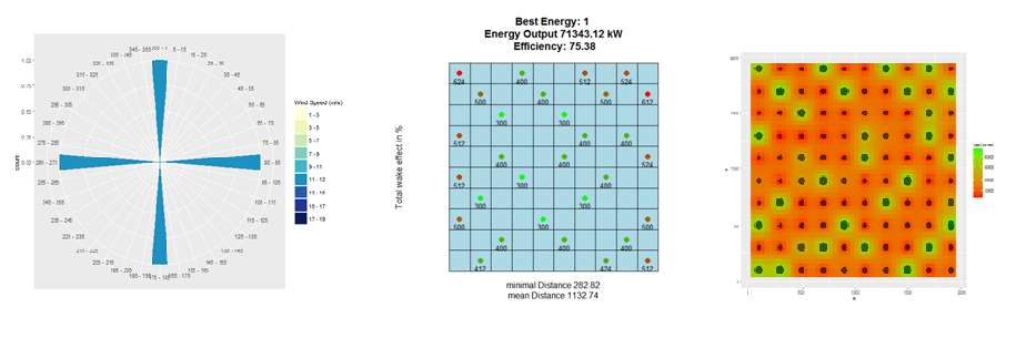
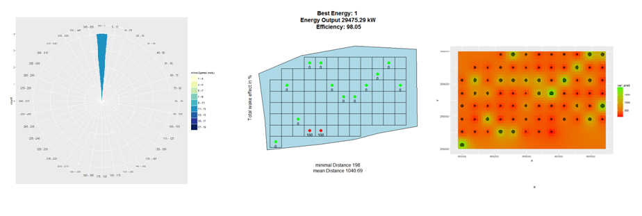
 - plot_windfarmGA(result, Polygon1)
 - plot_result(result, Polygon1, best = 1)
 - plot_evolution(result, ask = TRUE, spar = 0.1)
 - plot_development(result)
 - plot_parkfitness(result, spar = 0.1)
 - plot_fitness_evolution(result)
 - plot_cloud(result, pl = TRUE)
 - plot_heatmap(result = result, si = 5)
 - plot_leaflet(result = result, Polygon1 = Polygon1, which = 1)
A full documentation of the genetic algorithm is given in my master thesis.
Shiny Windfarm Optimization
I also made a Shiny App for the Genetic Algorithm. Unfortunately, as an optimization takes quite some time and the app is currently hosted by shinyapps.io under a public license, there is only 1 R-worker at hand. So only 1 optimization can be run at a time.
Full Optimization example:
library(sf)
library(windfarmGA)

Polygon1 <- sf::st_as_sf(sf::st_sfc(
  sf::st_polygon(list(cbind(
    c(4651704, 4651704, 4654475, 4654475, 4651704),
    c(2692925, 2694746, 2694746, 2692925, 2692925)))),
  crs = 3035
))
plot(Polygon1, col = "blue", axes = TRUE)

wind_df <- data.frame(ws = 12, wd = 0)
windrosePlot <- plot_windrose(data = wind_df, spd = wind_df$ws,
                             dir = wind_df$wd, dirres = 10, spdmax = 20)
Rotor <- 20
fcrR <- 9
Grid <- grid_area(shape = Polygon1, size = (Rotor*fcrR), prop = 1, plotGrid = TRUE)

result <- genetic_algorithm(Polygon1 = sp_polygon,
                            n = 20,
                            Rotor = Rotor, fcrR = fcrR,
                            iteration = 50,
                            vdirspe = wind_df,
                            referenceHeight = 50, RotorHeight = 100)

# The following function will execute all plotting function further below:
plot_windfarmGA(result, Polygon1, whichPl = "all", best = 1, plotEn = 1)

# The plotting functions can also be called individually:
plot_result(result, Polygon1, best = 1, plotEn = 1, topographie = FALSE)
plot_evolution(result, ask = TRUE, spar = 0.1)
plot_parkfitness(result, spar = 0.1)
plot_fitness_evolution(result)
plot_cloud(result, pl = TRUE)
plot_heatmap(result = result, si = 5)
plot_leaflet(result = result, Polygon1 = Polygon1, which = 1)